Splines |
When we remember the easy setup of polynomials, i.e.
Then we may ask isn’t it possible to define combined polynomials in a similar way? Because when building a movement out of say 3 combined 3rd order polynomials we actually would have 3 * 4 = 12 values to set. And this is a lot, so why not let an algorithm do the job for us?
A spline is a set of combined polynomials. When all polynomials are of 3rd order we call it a cubic spline, when of 5th order we call it a quintic spline and when of 7th order we call it a septic spline.
But let’s start simple by building a set of 3 segments each
of a 3rd order Polynomial 123 with each has Time = 1 s,
Start/End Velocity = ![]() and the first
Distance = 100 mm, the second Distance = -200 mm and the third
Distance = 100 mm.
and the first
Distance = 100 mm, the second Distance = -200 mm and the third
Distance = 100 mm.
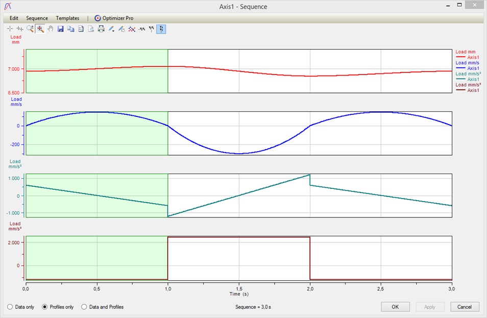
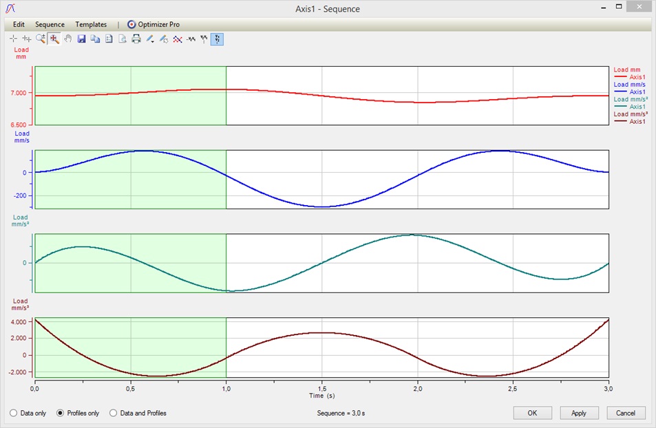
So when looking at the profiles we see that we have an acceleration jump at each junction of the 3 segments. This is because the polynomials are uniquely defined by the set variables above. Now in order to get rid of the acceleration jumps we usually would start playing with the Start/End Velocities at the junction points and this might be an annoying task to do manually.
Keeping in mind our simple polynomial approach, we can take advantage by using another Linear Algebra theorem.
This means in detail:
And we let the spline algorithms under the hood calculate a smooth curve at the junction points automatically.
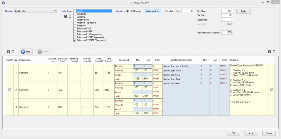
This task can simply be done by using the Optimizer with settings as shown here:
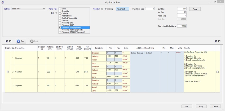
In this example, we don’t use the Optimizer to optimize for a
target. Instead we fix all free variables to our desired values
(for example setting the Duration of each segment fix to Min and
Max equal to 1 s and using the Additional Constraint “Spline:
Start Vel = End Vel” with also Min and Max fix to ![]() ).
).
Then let the Optimizer calculate a cubic spline with setting “Polynomial 123 (segments)” and “Population Size” set to zero (because no optimizing is needed).
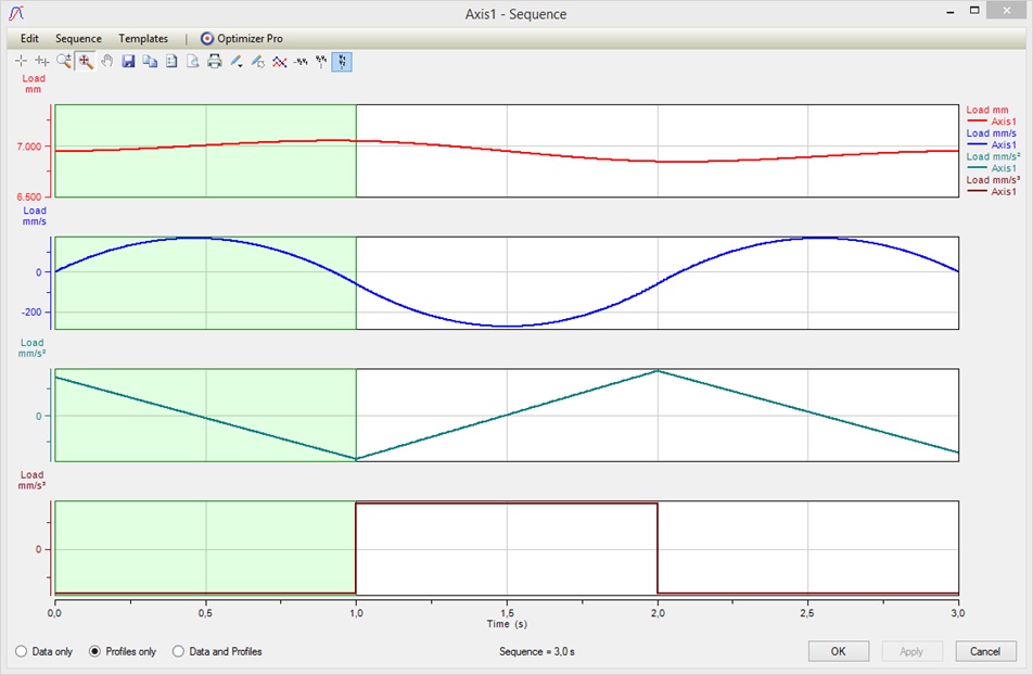
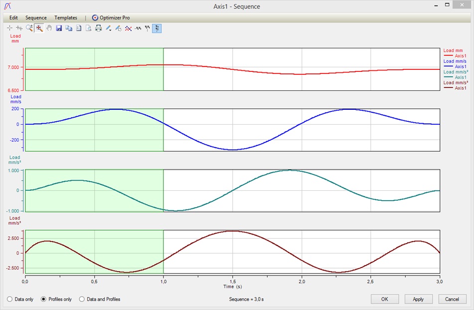
After applying our results we see that a unique cubic spline was calculated which is continuous in space, velocity and acceleration at each junction point, achieving an overall smooth movement:
Of course we can also use quintic splines to do the task.
Therefore we have to select “Polynomial 12345 (segments)” and
additionally have to set the Additional Constraints “Spline: Start
Accel” and “Spline: End Accel” with Min and Max accordingly fixed
to ![]() .
.
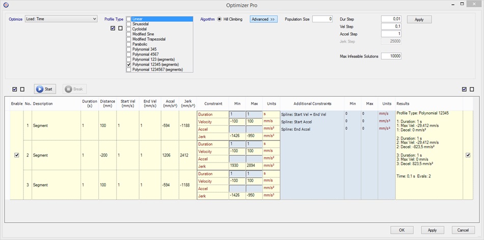
And with quintic splines further the 3rd derivative (“Jerk”) as well the 4th derivative (“Ping”, “Jounce” or “Snap”) are continous, allowing a more smoother movement than with cubic splines.
Last but not least we can use septic splines to do the task.
Therefore we have to select “Polynomial 1234567 (segments)” and
additionally have to set the Additional Constraints “Spline: Start
Jerk” and “Spline: End Jerk” with Min and Max accordingly fixed to
![]() .
.
And with septic splines further the 5th derivative (“Puff” or “Crackle”) as well the 6th derivative are continous, reducing vibrations, also allowing a jerk-free start and end of the movement.
What does the Optimizer actually do when calculating a spline?
Recall that a 3rd order polynomial is defined by
![]()
Where we have the four unknowns ![]() to solve for. So for
one 3rd order polynomial we have four equations to solve.
to solve for. So for
one 3rd order polynomial we have four equations to solve.
Considering a cubic spline with say 3 segments we will have then 3 * 4 = 12 equations to solve. But for a 3-segment cubic spline we have to set only 2 * 3 + 2 = 8 values (Times and Distances of each segment + Start/End Velocity of the whole spline).
So where do we get the missing 4 equations from?
We achieve them by demanding continuous first and second derivatives at the junction points. In our example above with each segment lasting 1 s this means for
| continuous velocities | |||
| and continuous accelerations |
Demanding this we now can setup a linear system of equations and solve it. In our example here there has to be a 12 x 12 matrix linear equation system solved.
In general:
Of course, this is all taken care of and solved numerically in the SERVOsoft Optimizer.